A Biased View of Vlookup Excel

By pushing ctrl+shift+center, this will calculate as well as return value from multiple arrays, as opposed to simply specific cells contributed to or multiplied by each other. Determining the sum, item, or quotient of specific cells is very easy-- just use the =AMOUNT formula as well as enter the cells, values, or series of cells you desire to carry out that math on.

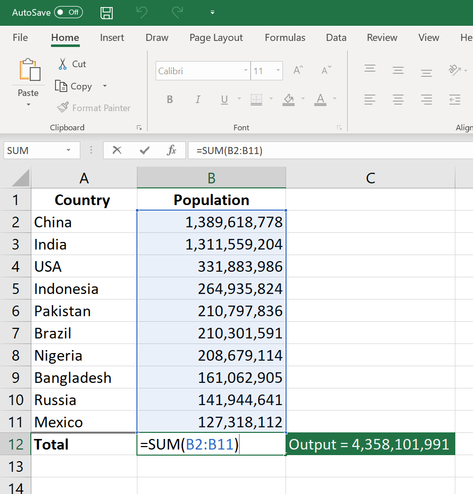
If you're wanting to locate overall sales revenue from a number of sold systems, for instance, the array formula in Excel is ideal for you. Here's just how you would certainly do it: To begin utilizing the array formula, kind "=SUM," and also in parentheses, enter the initial of 2 (or three, or 4) varieties of cells you want to multiply together.

This represents multiplication. Following this asterisk, enter your second range of cells. You'll be multiplying this second array of cells by the very first. Your progress in this formula should now resemble this: =AMOUNT(C 2: C 5 * D 2:D 5) Ready to push Get in? Not so fast ... Since this formula is so challenging, Excel books a various key-board command for ranges.

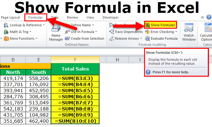
This will certainly acknowledge your formula as an array, wrapping your formula in support characters and effectively returning your item of both arrays incorporated. In income calculations, this can minimize your effort and time considerably. See the final formula in the screenshot above. The COUNT formula in Excel is denoted =COUNT(Beginning Cell: End Cell).

As an example, if there are eight cells with gone into values in between A 1 and A 10, =COUNT(A 1: A 10) will certainly return a worth of 8. The MATTER formula in Excel is especially valuable for big spreadsheets, wherein you wish to see the amount of cells include real access. Don't be fooled: This formula will not do any type of mathematics on the values of the cells themselves.

3 Simple Techniques For Excel If Formula

Making use of the formula in strong above, you can easily run a count of active cells in your spreadsheet. The outcome will certainly look a something similar to this: To perform the ordinary formula in Excel, get in the values, cells, or variety of cells of which you're calculating the standard in the layout, =AVERAGE(number 1, number 2, and so on) or =AVERAGE(Beginning Worth: End Worth).

Locating the standard of a series of cells in Excel keeps you from needing to discover individual amounts and afterwards carrying out a separate division formula on your total amount. Utilizing =AVERAGE as your first text entry, you can let Excel do all the job for you. For referral, the standard of a group of numbers is equivalent to the amount of those numbers, split by the number of things in that team.

This will certainly return the amount of the values within a preferred variety of cells that all fulfill one requirement. For instance, =SUMIF(C 3: C 12,"> 70,000") would certainly return the amount of values in between cells C 3 and also C 12 from just the cells that are more than 70,000. Allow's say you wish to identify the profit you produced from a checklist of leads that are related to details area codes, or compute the sum of specific workers' incomes-- but only if they fall over a specific quantity.

With the SUMIF feature, it doesn't need to be-- you can conveniently add up the amount of cells that satisfy particular criteria, like in the income instance above. The formula: =SUMIF(variety, requirements, [sum_range] Array: The variety that is being tested utilizing your criteria. Requirements: The requirements that identify which cells in Criteria_range 1 will certainly be totaled [Sum_range]: An optional variety of cells you're mosting likely to include up in addition to the very first Range got in.

In the example below, we wished to calculate the amount of the incomes that were above $70,000. The SUMIF feature built up the buck amounts that exceeded that number in the cells C 3 through C 12, with the formula =SUMIF(C 3: C 12,"> 70,000"). The TRIM formula in Excel is represented =TRIM(message).

6 Easy Facts About Learn Excel Described

For instance, if A 2 includes the name" Steve Peterson" with unwanted areas prior to the given name, =TRIM(A 2) would return "Steve Peterson" without any areas in a new cell. Email and also file sharing are terrific tools in today's office. That is, until one of your colleagues sends you a worksheet with some really cool spacing.

Instead than painstakingly removing as well as including spaces as required, you can tidy up any kind of irregular spacing using the TRIM function, which is utilized to remove added rooms from information (except for single rooms in between words). The formula: =TRIM(text). Text: The message or cell where you wish to get rid of spaces.

To do so, we entered =TRIM("A 2") right into the Formula Bar, and reproduced this for every name listed below it in a brand-new column beside the column with undesirable rooms. Below are a few other Excel formulas you may locate beneficial as your data administration requires grow. Let's say you have a line of text within a cell that you want to damage down into a few different segments.

Function: Used to remove the very first X numbers or characters in a cell. The formula: =LEFT(message, number_of_characters) Text: The string that you desire to draw out from. Number_of_characters: The number of characters that you desire to remove beginning from the left-most personality. In the example listed below, we went into =LEFT(A 2,4) right into cell B 2, and copied it into B 3: B 6.

Purpose: Made use of to remove characters or numbers in the center based upon position. The formula: =MID(text, start_position, number_of_characters) Text: The string that you desire to remove from. Start_position: The setting in the string that you intend to start removing from. As an example, the initial placement in the string is 1.

The 5-Second Trick For Excel Shortcuts

In this example, we entered =MID(A 2,5,2) right into cell B 2, and replicated it into B 3: B 6. That enabled us to extract the 2 numbers beginning in the fifth setting of the code. Purpose: Used to draw out the last X numbers or characters in a cell. The formula: =RIGHT(text, number_of_characters) Text: The string that you want to draw out from.

formulas excel not working formulas excel microsoft office excel formulas replace